The goal of this project is to develop an automated system for predicting loan eligibility based on customer details provided through an online application form. The company aims to streamline and optimize their loan approval process by leveraging data to identify customer segments that are most likely to be eligible for a loan. This will enable targeted marketing and more efficient processing of applications.

Problem Statement

The company has provided a dataset with customer information, including the following features: - Gender: The gender of the applicant. - Marital Status: Whether the applicant is married or not. - Education: The education level of the applicant. - Number of Dependents: The number of people financially dependent on the applicant. - Income: The applicant’s monthly income. - Loan Amount: The amount of loan applied for. - Credit History: A record of the applicant’s past credit behavior. - Others: Any additional relevant features.

The task is to use this data to identify which customers are eligible for a loan. This involves segmenting the customers into groups based on their likelihood of being approved for a loan. The dataset provided is partial, and the challenge is to work with the available data to build a predictive model.

Importing Libraries

import  numpy as np
import  pandas as pd
import seaborn as sns
import matplotlib.pyplot as plt
%matplotlib inline

from sklearn.model_selection import train_test_split
from sklearn import feature_selection
from sklearn import model_selection
from sklearn.metrics import accuracy_score 
from sklearn.linear_model import LogisticRegression
from sklearn.svm import SVC
from sklearn.naive_bayes import GaussianNB
from sklearn.ensemble import RandomForestClassifier,GradientBoostingClassifier
from sklearn.neighbors import KNeighborsClassifier

import warnings
warnings.filterwarnings('ignore')

Importing data

train = pd.read_csv('../input/loan-prediction-problem-dataset/train_u6lujuX_CVtuZ9i.csv')
test = pd.read_csv('../input/loan-prediction-problem-dataset/test_Y3wMUE5_7gLdaTN.csv')

print (train.shape, test.shape)

(614, 13) (367, 12)

Data Exploration

train.head()

	Loan_ID	Gender	Married	Dependents	Education	Self_Employed	ApplicantIncome	CoapplicantIncome	LoanAmount	Loan_Amount_Term	Credit_History	Property_Area	Loan_Status
0	LP001002	Male	No	0	Graduate	No	5849	0.0	NaN	360.0	1.0	Urban	Y
1	LP001003	Male	Yes	1	Graduate	No	4583	1508.0	128.0	360.0	1.0	Rural	N
2	LP001005	Male	Yes	0	Graduate	Yes	3000	0.0	66.0	360.0	1.0	Urban	Y
3	LP001006	Male	Yes	0	Not Graduate	No	2583	2358.0	120.0	360.0	1.0	Urban	Y
4	LP001008	Male	No	0	Graduate	No	6000	0.0	141.0	360.0	1.0	Urban	Y

train.info()

<class 'pandas.core.frame.DataFrame'>
RangeIndex: 614 entries, 0 to 613
Data columns (total 13 columns):
 #   Column             Non-Null Count  Dtype  
---  ------             --------------  -----  
 0   Loan_ID            614 non-null    object 
 1   Gender             601 non-null    object 
 2   Married            611 non-null    object 
 3   Dependents         599 non-null    object 
 4   Education          614 non-null    object 
 5   Self_Employed      582 non-null    object 
 6   ApplicantIncome    614 non-null    int64  
 7   CoapplicantIncome  614 non-null    float64
 8   LoanAmount         592 non-null    float64
 9   Loan_Amount_Term   600 non-null    float64
 10  Credit_History     564 non-null    float64
 11  Property_Area      614 non-null    object 
 12  Loan_Status        614 non-null    object 
dtypes: float64(4), int64(1), object(8)
memory usage: 62.5+ KB

train.isnull().sum()

Loan_ID               0
Gender               13
Married               3
Dependents           15
Education             0
Self_Employed        32
ApplicantIncome       0
CoapplicantIncome     0
LoanAmount           22
Loan_Amount_Term     14
Credit_History       50
Property_Area         0
Loan_Status           0
dtype: int64

test.head()

	Loan_ID	Gender	Married	Dependents	Education	Self_Employed	ApplicantIncome	CoapplicantIncome	LoanAmount	Loan_Amount_Term	Credit_History	Property_Area
0	LP001015	Male	Yes	0	Graduate	No	5720	0	110.0	360.0	1.0	Urban
1	LP001022	Male	Yes	1	Graduate	No	3076	1500	126.0	360.0	1.0	Urban
2	LP001031	Male	Yes	2	Graduate	No	5000	1800	208.0	360.0	1.0	Urban
3	LP001035	Male	Yes	2	Graduate	No	2340	2546	100.0	360.0	NaN	Urban
4	LP001051	Male	No	0	Not Graduate	No	3276	0	78.0	360.0	1.0	Urban

test.info()

<class 'pandas.core.frame.DataFrame'>
RangeIndex: 367 entries, 0 to 366
Data columns (total 12 columns):
 #   Column             Non-Null Count  Dtype  
---  ------             --------------  -----  
 0   Loan_ID            367 non-null    object 
 1   Gender             356 non-null    object 
 2   Married            367 non-null    object 
 3   Dependents         357 non-null    object 
 4   Education          367 non-null    object 
 5   Self_Employed      344 non-null    object 
 6   ApplicantIncome    367 non-null    int64  
 7   CoapplicantIncome  367 non-null    int64  
 8   LoanAmount         362 non-null    float64
 9   Loan_Amount_Term   361 non-null    float64
 10  Credit_History     338 non-null    float64
 11  Property_Area      367 non-null    object 
dtypes: float64(3), int64(2), object(7)
memory usage: 34.5+ KB

test.isnull().sum()

Loan_ID               0
Gender               11
Married               0
Dependents           10
Education             0
Self_Employed        23
ApplicantIncome       0
CoapplicantIncome     0
LoanAmount            5
Loan_Amount_Term      6
Credit_History       29
Property_Area         0
dtype: int64

Data Preparation / Processing

data = [train,test]
for dataset in data:
    #Filter categorical variables
    categorical_columns = [x for x in dataset.dtypes.index if dataset.dtypes[x]=='object']
    # Exclude ID cols and source:
    categorical_columns = [x for x in categorical_columns if x not in ['Loan_ID' ]]
    #Print frequency of categories
    
for col in categorical_columns:
    print ('\nFrequency of Categories for variable %s'%col)
    print (train[col].value_counts())


Frequency of Categories for variable Gender
Gender
Male      489
Female    112
Name: count, dtype: int64

Frequency of Categories for variable Married
Married
Yes    398
No     213
Name: count, dtype: int64

Frequency of Categories for variable Dependents
Dependents
0     345
1     102
2     101
3+     51
Name: count, dtype: int64

Frequency of Categories for variable Education
Education
Graduate        480
Not Graduate    134
Name: count, dtype: int64

Frequency of Categories for variable Self_Employed
Self_Employed
No     500
Yes     82
Name: count, dtype: int64

Frequency of Categories for variable Property_Area
Property_Area
Semiurban    233
Urban        202
Rural        179
Name: count, dtype: int64

Gender

sns.countplot(train['Gender'])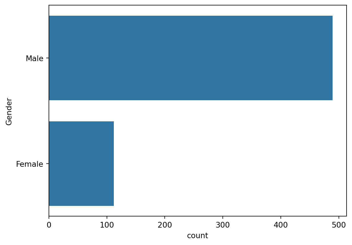

pd.crosstab(train.Gender, train.Loan_Status, margins = True)

Loan_Status	N	Y	All
Gender
Female	37	75	112
Male	150	339	489
All	187	414	601

The male are in large number as compared to female applicants.Also many of them have positive Loan Status. Further Binarization of this feature should be done,

train.Gender = train.Gender.fillna(train.Gender.mode())
test.Gender = test.Gender.fillna(test.Gender.mode())

sex = pd.get_dummies(train['Gender'] , drop_first = True )
train.drop(['Gender'], axis = 1 , inplace =True)
train = pd.concat([train , sex ] , axis = 1)

sex = pd.get_dummies(test['Gender'] , drop_first = True )
test.drop(['Gender'], axis = 1 , inplace =True)
test = pd.concat([test , sex ] , axis = 1)

Dependants

plt.figure(figsize=(6,6))
labels = ['0' , '1', '2' , '3+']
explode = (0.05, 0, 0, 0)
size = [345 , 102 , 101 , 51]

plt.pie(size, explode=explode, labels=labels,
        autopct='%1.1f%%', shadow = True, startangle = 90)
plt.axis('equal')
plt.show()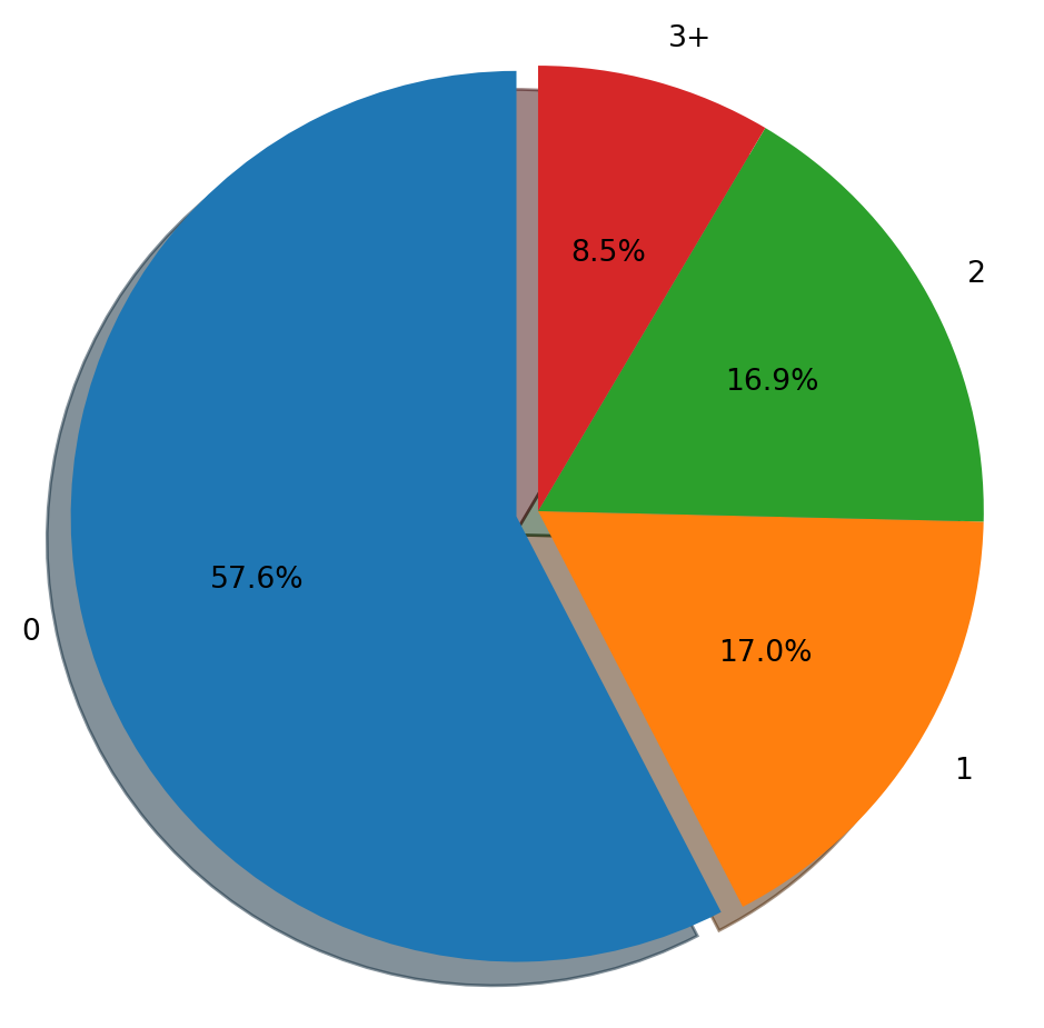

train.Dependents.value_counts()

Dependents
0     345
1     102
2     101
3+     51
Name: count, dtype: int64

pd.crosstab(train.Dependents , train.Loan_Status, margins = True)

Loan_Status	N	Y	All
Dependents
0	107	238	345
1	36	66	102
2	25	76	101
3+	18	33	51
All	186	413	599

The applicants with highest number of dependants are least in number whereas applicants with no dependance are greatest among these.

train.Dependents = train.Dependents.fillna("0")
test.Dependents = test.Dependents.fillna("0")

rpl = {'0':'0', '1':'1', '2':'2', '3+':'3'}

train.Dependents = train.Dependents.replace(rpl).astype(int)
test.Dependents = test.Dependents.replace(rpl).astype(int)

Credit History

pd.crosstab(train.Credit_History , train.Loan_Status, margins = True)

Loan_Status	N	Y	All
Credit_History
0.0	82	7	89
1.0	97	378	475
All	179	385	564

train.Credit_History = train.Credit_History.fillna(train.Credit_History.mode()[0])
test.Credit_History  = test.Credit_History.fillna(test.Credit_History.mode()[0])

Self Employed

sns.countplot(train['Self_Employed'])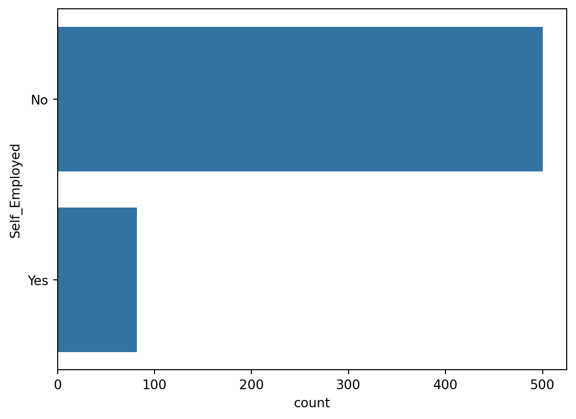

pd.crosstab(train.Self_Employed , train.Loan_Status,margins = True)

Loan_Status	N	Y	All
Self_Employed
No	157	343	500
Yes	26	56	82
All	183	399	582

train.Self_Employed = train.Self_Employed.fillna(train.Self_Employed.mode())
test.Self_Employed = test.Self_Employed.fillna(test.Self_Employed.mode())

self_Employed = pd.get_dummies(train['Self_Employed'] ,prefix = 'employed' ,drop_first = True )
train.drop(['Self_Employed'], axis = 1 , inplace =True)
train = pd.concat([train , self_Employed ] , axis = 1)

self_Employed = pd.get_dummies(test['Self_Employed'] , prefix = 'employed' ,drop_first = True )
test.drop(['Self_Employed'], axis = 1 , inplace =True)
test = pd.concat([test , self_Employed ] , axis = 1)

Married

sns.countplot(train.Married)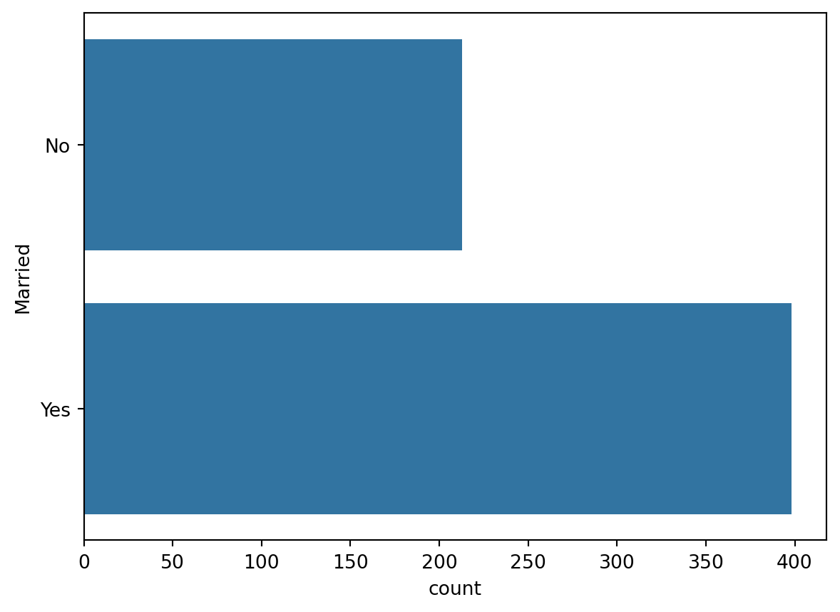

pd.crosstab(train.Married , train.Loan_Status,margins = True)

Loan_Status	N	Y	All
Married
No	79	134	213
Yes	113	285	398
All	192	419	611

train.Married = train.Married.fillna(train.Married.mode())
test.Married = test.Married.fillna(test.Married.mode())

married = pd.get_dummies(train['Married'] , prefix = 'married',drop_first = True )
train.drop(['Married'], axis = 1 , inplace =True)
train = pd.concat([train , married ] , axis = 1)

married = pd.get_dummies(test['Married'] , prefix = 'married', drop_first = True )
test.drop(['Married'], axis = 1 , inplace =True)
test = pd.concat([test , married ] , axis = 1)

Loan Amount Term and Loan Amount

train.drop(['Loan_Amount_Term'], axis = 1 , inplace =True)
test.drop(['Loan_Amount_Term'], axis = 1 , inplace =True)

train.LoanAmount = train.LoanAmount.fillna(train.LoanAmount.mean()).astype(int)
test.LoanAmount = test.LoanAmount.fillna(test.LoanAmount.mean()).astype(int)

sns.distplot(train['LoanAmount'])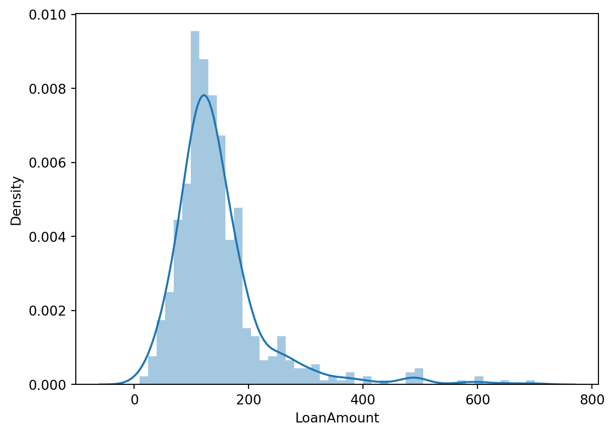

We observe no outliers in the continuous variable Loan Amount

Education

sns.countplot(train.Education)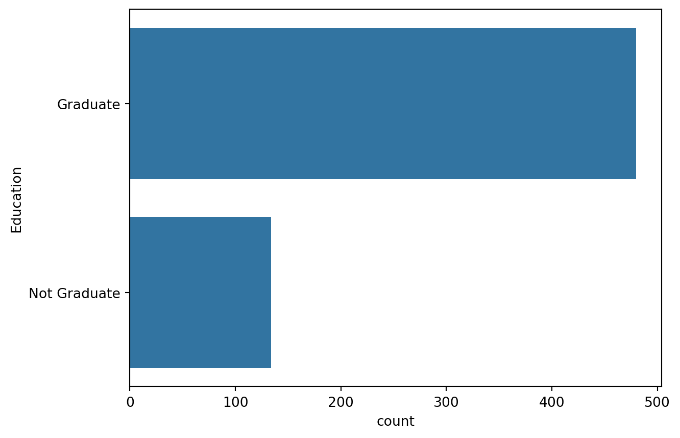

train['Education'] = train['Education'].map( {'Graduate': 0, 'Not Graduate': 1} ).astype(int)
test['Education'] = test['Education'].map( {'Graduate': 0, 'Not Graduate': 1} ).astype(int)

Property Area

sns.countplot(train.Property_Area)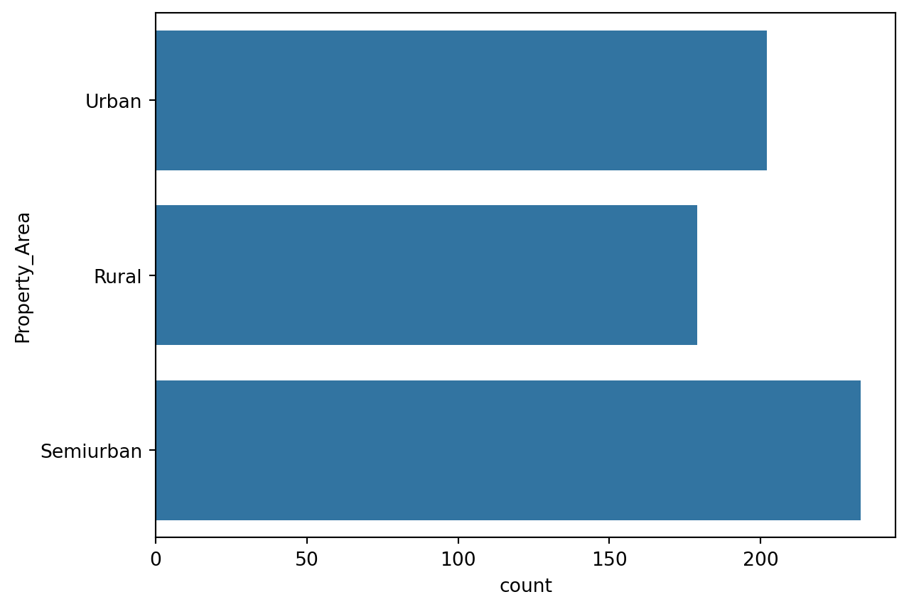

train['Property_Area'] = train['Property_Area'].map( {'Urban': 0, 'Semiurban': 1 ,'Rural': 2  } ).astype(int)

test.Property_Area = test.Property_Area.fillna(test.Property_Area.mode())
test['Property_Area'] = test['Property_Area'].map( {'Urban': 0, 'Semiurban': 1 ,'Rural': 2  } ).astype(int)

Co-Applicant income and Applicant income

sns.distplot(train['ApplicantIncome'])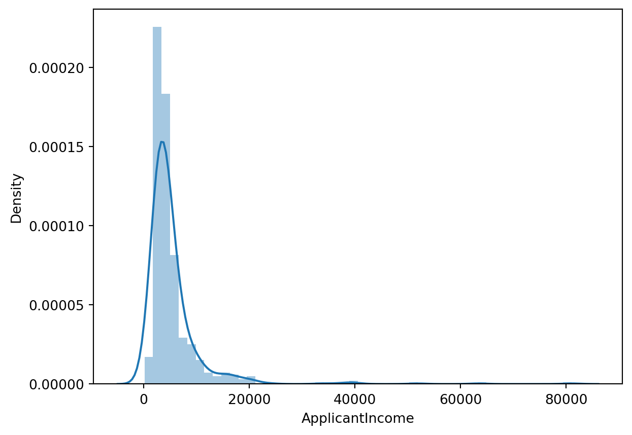

sns.distplot(train['CoapplicantIncome'])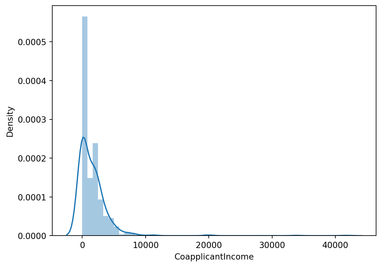

Target Variable : Loan Status

train['Loan_Status'] = train['Loan_Status'].map( {'N': 0, 'Y': 1 } ).astype(int)

Dropping the ID column

train.drop(['Loan_ID'], axis = 1 , inplace =True)

View the datasets

train.head()

	Dependents	Education	ApplicantIncome	CoapplicantIncome	LoanAmount	Credit_History	Property_Area	Loan_Status	Male	employed_Yes	married_Yes
0	0	0	5849	0.0	146	1.0	0	1	True	False	False
1	1	0	4583	1508.0	128	1.0	2	0	True	False	True
2	0	0	3000	0.0	66	1.0	0	1	True	True	True
3	0	1	2583	2358.0	120	1.0	0	1	True	False	True
4	0	0	6000	0.0	141	1.0	0	1	True	False	False

test.head()

	Loan_ID	Dependents	Education	ApplicantIncome	CoapplicantIncome	LoanAmount	Credit_History	Male	employed_Yes	married_Yes
0	LP001015	0	0	5720	0	110	1.0	True	False	True
1	LP001022	1	0	3076	1500	126	1.0	True	False	True
2	LP001031	2	0	5000	1800	208	1.0	True	False	True
3	LP001035	2	0	2340	2546	100	1.0	True	False	True
4	LP001051	0	1	3276	0	78	1.0	True	False	False

Visualizing the correlations and relation

Plot between LoanAmount, Applicant Income, Employement and Gender

What is the relation of Loan taken between men and women?
Did the employed ones were greater in number to take Loan ?
What is distribution of Loan Amount and Income?

# Corrected code using height instead of size
g = sns.lmplot(x='ApplicantIncome', y='LoanAmount', data=train, col='employed_Yes', hue='Male',
               palette=["Red", "Blue", "Yellow"], aspect=1.2, height=3)
g.set(ylim=(0, 800))
# Relation between the male or female applicant's income, loan taken, and self-employment status.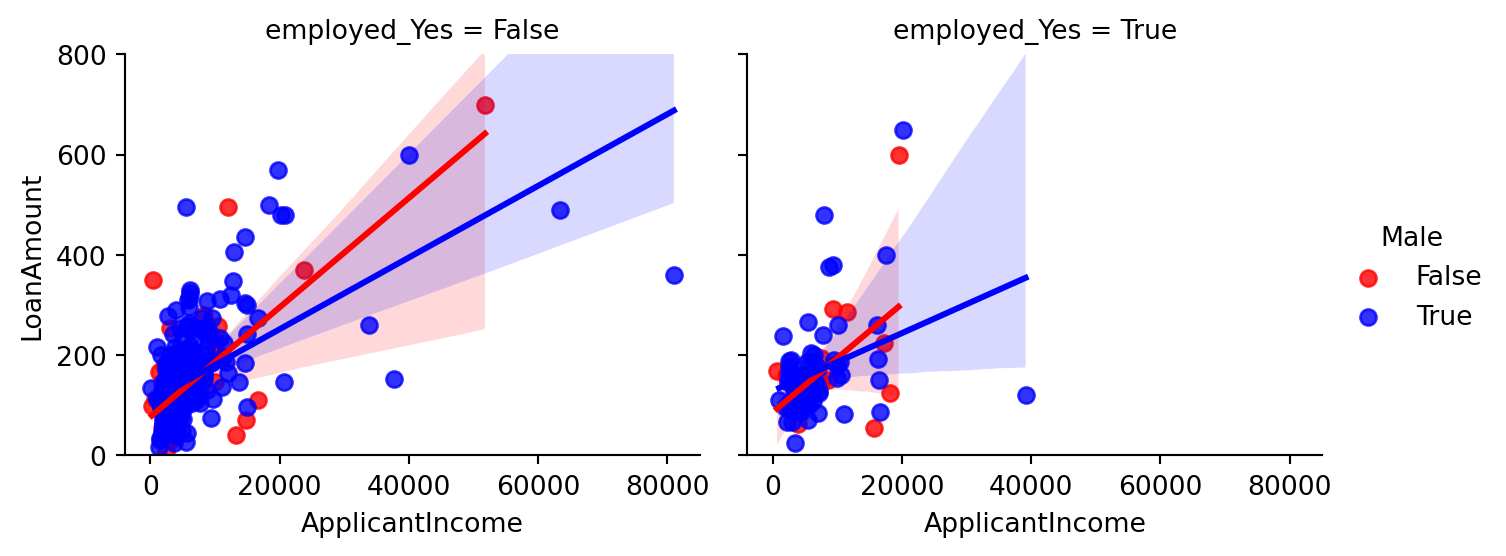

Above graph tells:
- The male applicants take more amount of loan than female.
- The males are higher in number of “NOT self employed” category.
- The amount is still larger in the income range in (0 to 20000).
- Also we observe that majority of applicants are NOT self employed.
- Highest Loan amount taken is by the female applicant of about 700 which is NOT self employed.
- The majority of income taken is about 0-200 with income in the range 0-20000.
- The line plotted shows that with increase in income the amount of loan increases with almost same slope for the case of women in both the cases but a slightely lesser slope in the case of men in Self- Employed category as compared to non-self employed.

Boxplots for relation between Property area, amount of Loan and Education qualification

Further we analyse the relation between education status,loan taken and property area

Property_Area:
- Urban :0
- Semiurban :1
- Rural :2

plt.figure(figsize=(5,2))
sns.boxplot(x="Property_Area", y="LoanAmount", hue="Education",data=train, palette="coolwarm")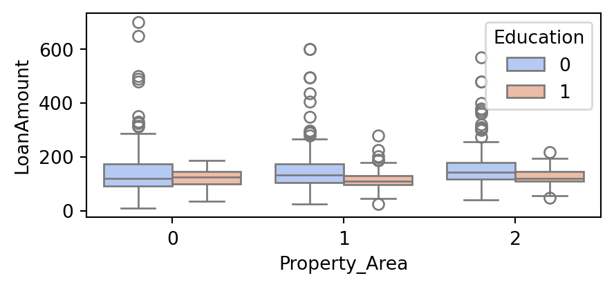

The above boxplot signifies that,
- In the Urban area the non graduates take slightly more loan than graduates.
- In the Rural and semiurban area the graduates take more amount of Loan than non graduates
- The higher values of Loan are mostly from Urban area
- The semiurban area and rural area both have one unusual Loan amount close to zero.

Crosstab for relation between Credit History and Loan status.

train.Credit_History.value_counts()

Credit_History
1.0    525
0.0     89
Name: count, dtype: int64

lc = pd.crosstab(train['Credit_History'], train['Loan_Status'])
lc.plot(kind='bar', stacked=True, color=['red','blue'], grid=False)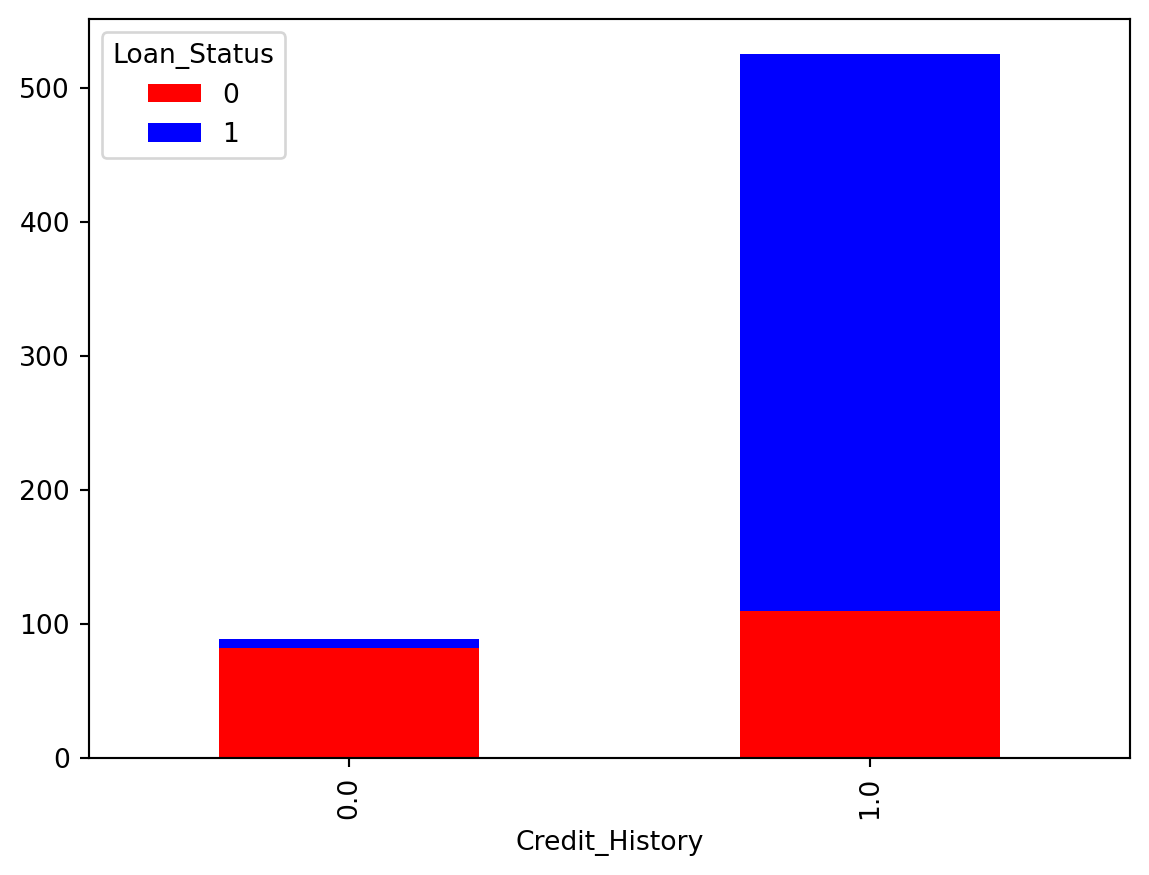

The credit history vs Loan Status indicates:
- The good credit history applicants have more chances of getting Loan.
- With better credit History the Loan amount given was greater too.
- But many were not given loan in the range 0-100
- The applicant with poor credit history were handled in the range 0-100 only.

plt.figure(figsize=(9,6))
sns.heatmap(train.drop('Loan_Status',axis=1).corr(), vmax=0.6, square=True, annot=True)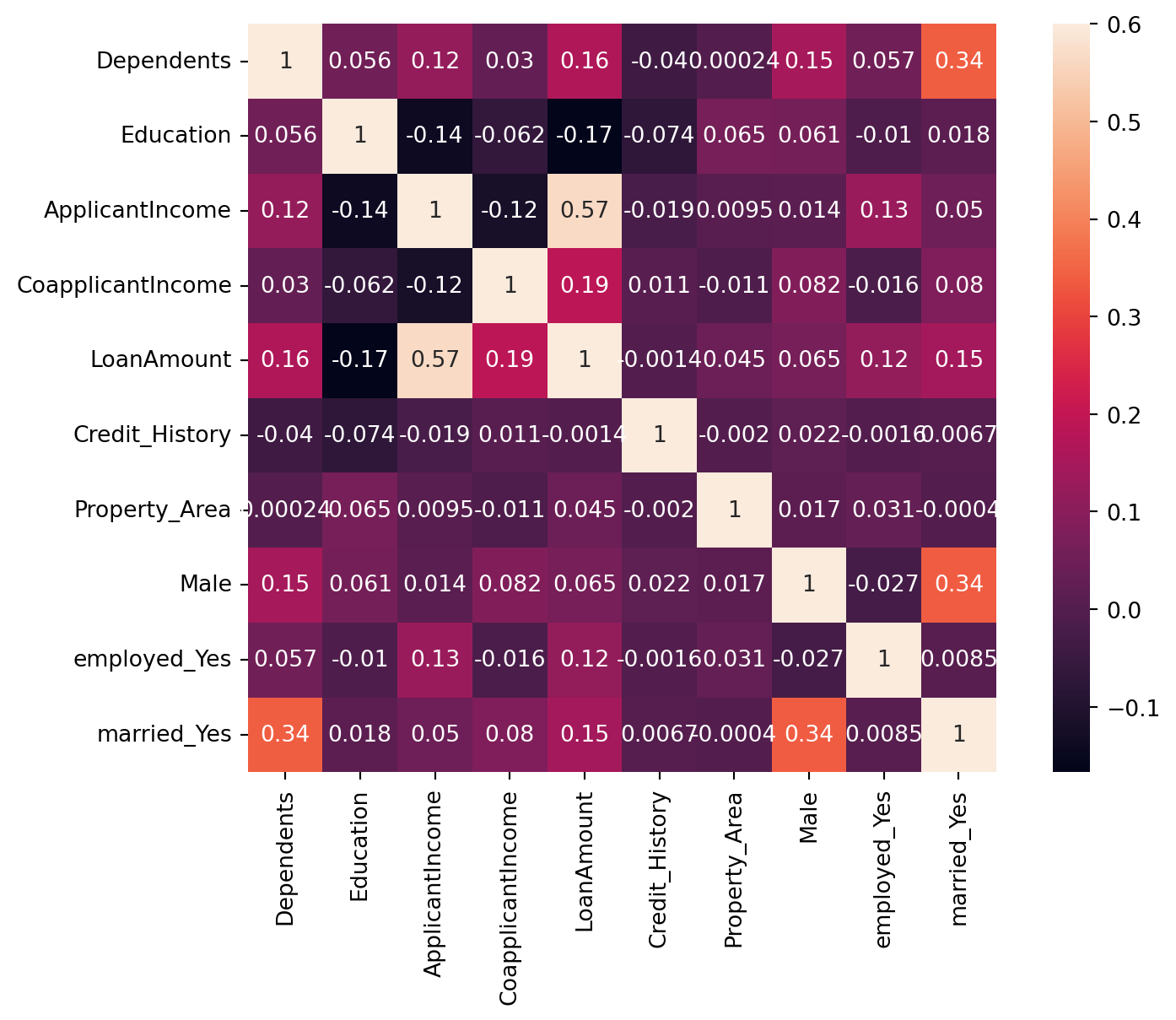

Prediction

The problem is of Classification as observed and concluded from the data and visualisations.

X = train.drop('Loan_Status' , axis = 1 )
y = train['Loan_Status']

X_train ,X_test , y_train , y_test = train_test_split(X , y , test_size = 0.3 , random_state =102)

from sklearn.linear_model import LogisticRegression
logmodel = LogisticRegression()
logmodel.fit(X_train , y_train)
pred_l = logmodel.predict(X_test)
acc_l = accuracy_score(y_test , pred_l)*100
acc_l

83.78378378378379

random_forest = RandomForestClassifier(n_estimators= 100)
random_forest.fit(X_train, y_train)
pred_rf = random_forest.predict(X_test)
acc_rf = accuracy_score(y_test , pred_rf)*100
acc_rf

80.54054054054053

knn = KNeighborsClassifier(n_neighbors = 3)
knn.fit(X_train, y_train)
pred_knn = knn.predict(X_test)
acc_knn = accuracy_score(y_test , pred_knn)*100
acc_knn

61.08108108108108

gaussian = GaussianNB()
gaussian.fit(X_train, y_train)
pred_gb = gaussian.predict(X_test)
acc_gb = accuracy_score(y_test , pred_gb)*100
acc_gb

82.16216216216216

svc = SVC()
svc.fit(X_train, y_train)
pred_svm = svc.predict(X_test)
acc_svm = accuracy_score(y_test , pred_svm)*100
acc_svm

70.27027027027027

gbk = GradientBoostingClassifier()
gbk.fit(X_train, y_train)
pred_gbc = gbk.predict(X_test)
acc_gbc = accuracy_score(y_test , pred_gbc)*100
acc_gbc

82.16216216216216

## Arranging the Accuracy results
models = pd.DataFrame({
    'Model': ['Logistic Regression', 'Random Forrest','K- Nearest Neighbour' ,
             'Naive Bayes' , 'SVM','Gradient Boosting Classifier'],
    'Score': [acc_l , acc_rf , acc_knn , acc_gb ,acc_svm ,acc_gbc ]})
models.sort_values(by='Score', ascending=False)

	Model	Score
0	Logistic Regression	83.783784
3	Naive Bayes	82.162162
5	Gradient Boosting Classifier	82.162162
1	Random Forrest	80.540541
4	SVM	70.270270
2	K- Nearest Neighbour	61.081081

The highest classification accuracy is shown by Logistic Regression of about 83.24 %

Let us Check th feature importance,

importances = pd.DataFrame({'Features':X_train.columns,'Importance':np.round(random_forest.feature_importances_,3)})
importances = importances.sort_values('Importance',ascending=False).set_index('Features')
importances.head(11)

	Importance
Features
Credit_History	0.248
ApplicantIncome	0.216
LoanAmount	0.211
CoapplicantIncome	0.122
Dependents	0.053
Property_Area	0.052
Education	0.027
married_Yes	0.026
Male	0.024
employed_Yes	0.021

importances.plot.bar()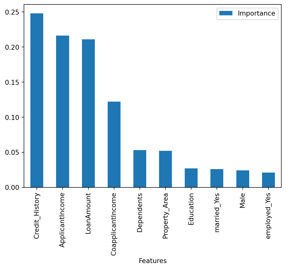

Credit History has the maximum importance and empoloyment has the least!

Summarizing

The Loan status has better relation with features such as Credit History, Applicant’s Income, Loan Amount needed by them, Family status(Depenedents) and Property Area which are generally considered by the loan providing organisations. These factors are hence used to take correct decisions to provide loan status or not. This data analysis hence gives a realisation of features and the relation between them from the older decision examples hence giving a learning to predict the class of the unseen data.

Finally the we predict over unseen dataset using the Logistic Regression and Random Forest model(Ensemble Learning):

df_test = test.drop(['Loan_ID'], axis = 1)

df_test.head()

	Dependents	Education	ApplicantIncome	CoapplicantIncome	LoanAmount	Credit_History	Male	employed_Yes	married_Yes
0	0	0	5720	0	110	1.0	True	False	True
1	1	0	3076	1500	126	1.0	True	False	True
2	2	0	5000	1800	208	1.0	True	False	True
3	2	0	2340	2546	100	1.0	True	False	True
4	0	1	3276	0	78	1.0	True	False	False

p_log = logmodel.predict(df_test)

p_rf = random_forest.predict(df_test)

predict_combine = np.zeros((df_test.shape[0]))

for i in range(0, test.shape[0]):
    temp = p_log[i] + p_rf[i]
    if temp>=2:
        predict_combine[i] = 1
predict_combine = predict_combine.astype('int')

submission = pd.DataFrame({
        "Loan_ID": test["Loan_ID"],
        "Loan_Status": predict_combine
    })

submission.to_csv("results.csv", encoding='utf-8', index=False)

Thank you

Author: Pratik Kumar